Related publications: [KNPS19]
In this case study, we consider a scenario in which two robots move concurrently over a grid of size l×l for some l>0. The robots start in diagonally opposite corners and try to reach the opposite corner from which they start. A robot can move either diagonally, horizontally or vertically towards its goal and when it moves there is a probability (q) that it instead moves in an adjacent direction, due to the presence of an obstacle. For example, if a robot tries to move north west, then with probability q/2 it will move north or west.
The PRISM code representing a concurrent stochastic game (CSG) model of this scenario is given below. The model has two parameters: l the size of the grid and q the probability of a movement failure. There are two players corresponding to the two robots and one module for each player.
The PRISM model also includes a reward structure for each player corresponding to elapsed time. These assume that it takes one time step to move between grid squares, except that after a crash (i.e., when the two robots end up in the same square) it take 10 time units to move squares.
// Two robots moving over a grid
// One tries to move from the SW corner to the NE corner while the other does the reverse
// When moving, a robot can end up in an adjacent grid square with probability q

// concurrent game model
csg

// the players
player robot1 robot1 endplayer
player robot2 robot2 endplayer

const double q; // probability of movement failure
const int l; // size of grid

// corner points
const int xmin = 0;
const int ymin = 0;
const int xmax = l-1;
const int ymax = l-1;

// initial grid positions for the robots
const int xi1 = xmin; const int yi1 = ymin;
const int xi2 = xmax; const int yi2 = ymax;

// goal grid positions for the robots
const int xg1 = xmax; const int yg1 = ymax;
const int xg2 = xmin; const int yg2 = ymin;

// add labels for specifying properties
label "goal1" = x1=xg1 & y1=yg1;
label "goal2" = x2=xg2 & y2=yg2;

// robots crash when they end up in same grid square
label "crash" = x1=x2 & y1=y2;

// first robot
module robot1

	x1 : [xmin..xmax] init xi1; // x coordinate
	y1 : [ymin..ymax] init yi1; // y coordinate

	[n1] y1<ymax -> (1-q) : (y1'=y1+1) + q/2 : (y1'=y1+1) & (x1'=min(xmax,x1+1)) + q/2 : (y1'=y1+1) & (x1'=max(xmin,x1-1));
	[e1] x1<xmax -> (1-q) : (x1'=x1+1) + q/2 : (x1'=x1+1) & (y1'=min(ymax,y1+1)) + q/2 : (x1'=x1+1) & (y1'=max(ymin,y1-1));
	[ne1] y1<ymax & x1<xmax -> (1-q) : (y1'=y1+1) & (x1'=x1+1) + q/2 : (y1'=y1+1) + q/2 : (x1'=x1+1);

	[done1] y1=yg1 & x1=xg1 -> true;

endmodule

// second robot
module robot2

	x2 : [xmin..xmax] init xi2; // x coordinate
	y2 : [ymin..ymax] init yi2; // y coordinate

	[s2] y2>ymin -> (1-q) : (y2'=y2-1) + q/2 : (y2'=y2-1) & (x2'=min(xmax,x2+1)) + q/2 : (y2'=y2-1) & (x2'=max(xmin,x2-1));
	[w2] x2>xmin -> (1-q) : (x2'=x2-1) + q/2 : (x2'=x2-1) & (y2'=min(ymax,y2+1)) + q/2 : (x2'=x2-1) & (y2'=max(ymin,y2-1));
	[sw2] y2>ymin & x2>xmin -> (1-q) : (y2'=y2-1) & (x2'=x2-1) + q/2 : (y2'=y2-1) + q/2 : (x2'=x2-1);

	[done2] y2=yg2 & x2=xg2 -> true;

endmodule

// rewards for robot 1
rewards "time1"
	[] !(x1=x2 & y1=y2) & !(y1=yg1 & x1=xg1) : 1;
	[] x1=x2 & y1=y2 & !(y1=yg1 & x1=xg1) : 10; // recovering from a crash takes 10 time units
endrewards

// rewards for robot 2
rewards "time2"
	[] !(x1=x2 & y1=y2) & !(y2=yg2 & x2=xg2) : 1;
	[] x1=x2 & y1=y2 & !(y2=yg2 & x2=xg2) : 10; // recovering from a crash takes 10 time units
endrewards
We first consider zero-sum properties in which the first player (robot) tries to achieve some goal and the second tries to prevent the first player from achieving this goal. We consider the following properties:
These properties are formally specified as follows.
const int k; // step bound

// maximum probability robot 1 can guarantee to reach its goal without crashing
<<robot1>>Pmax=? [ !"crash" U "goal1" ]

// maximum probability robot 1 can guarantee to reach its goal without crashing within a deadline
<<robot1>>Pmax=? [ !"crash" U<=k "goal1" ]

// minimum expected time robot 1 can guarantee to reach its goal
<<robot1>>R{"time1"}min=? [ F "goal1" ]
The following graph plots, for varying q and l, the maximum probability that player 1 can guarantee for eventually reaching its goal without crashing,
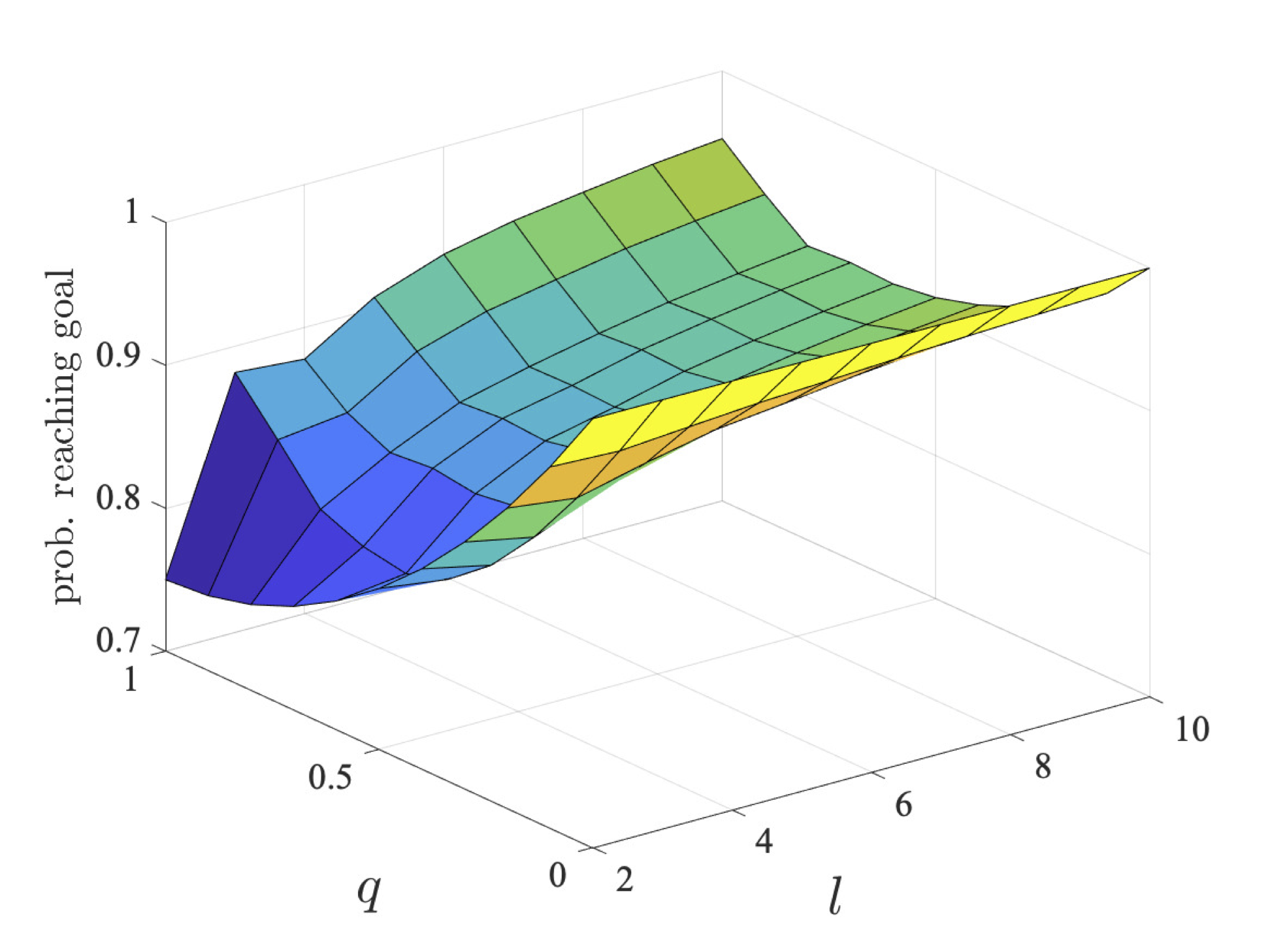
The results demonstrate that the probability increases as the size of the grid increases, which follows from the fact for larger grids it is easier to avoid the other robot, and hence not crash. On the other hand, as the probability of a movement failure increases, the probability of reaching the goal without crashing decreases since it is difficult to avoid crashing with more limited control of movement. As the size of the grid increases and this probability increases, after the initial decrease, the probability then increases as given a large area and the second robot having less control of movement, the first can avoid crashing even with its limited control of movement.
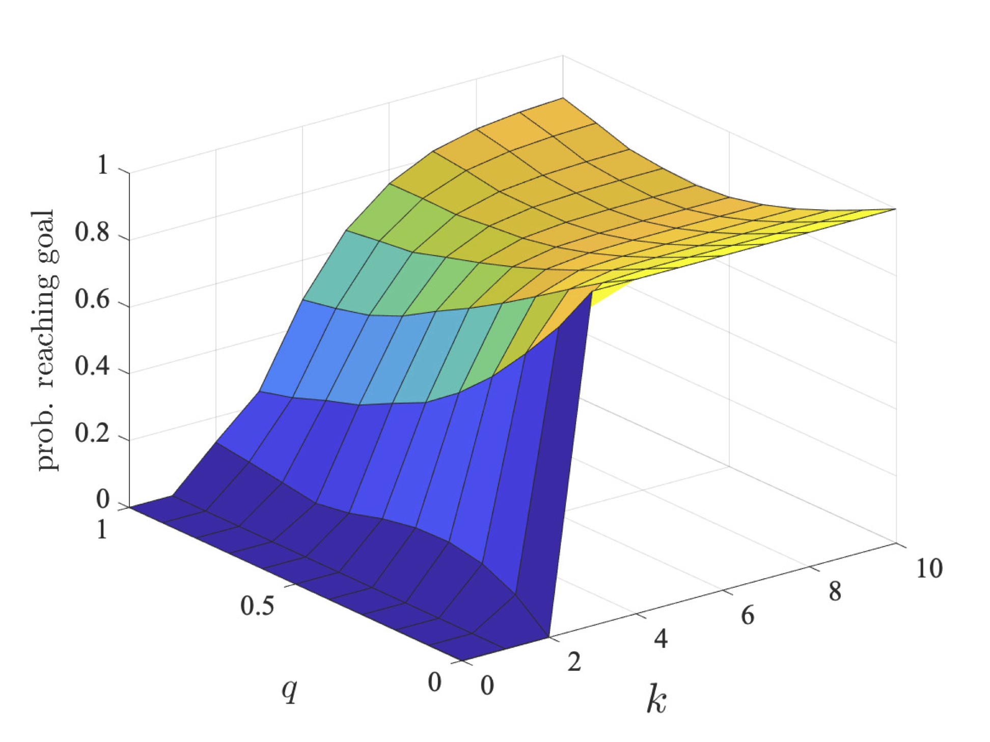
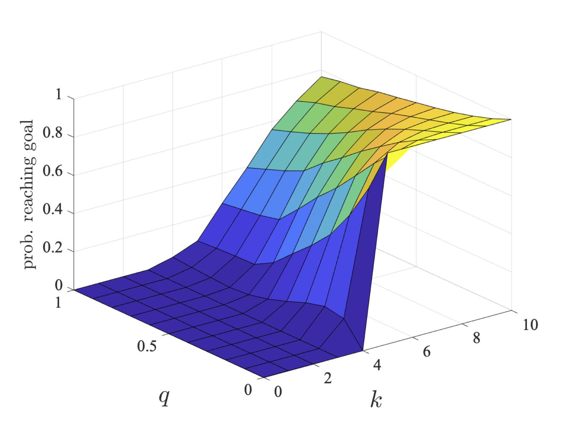
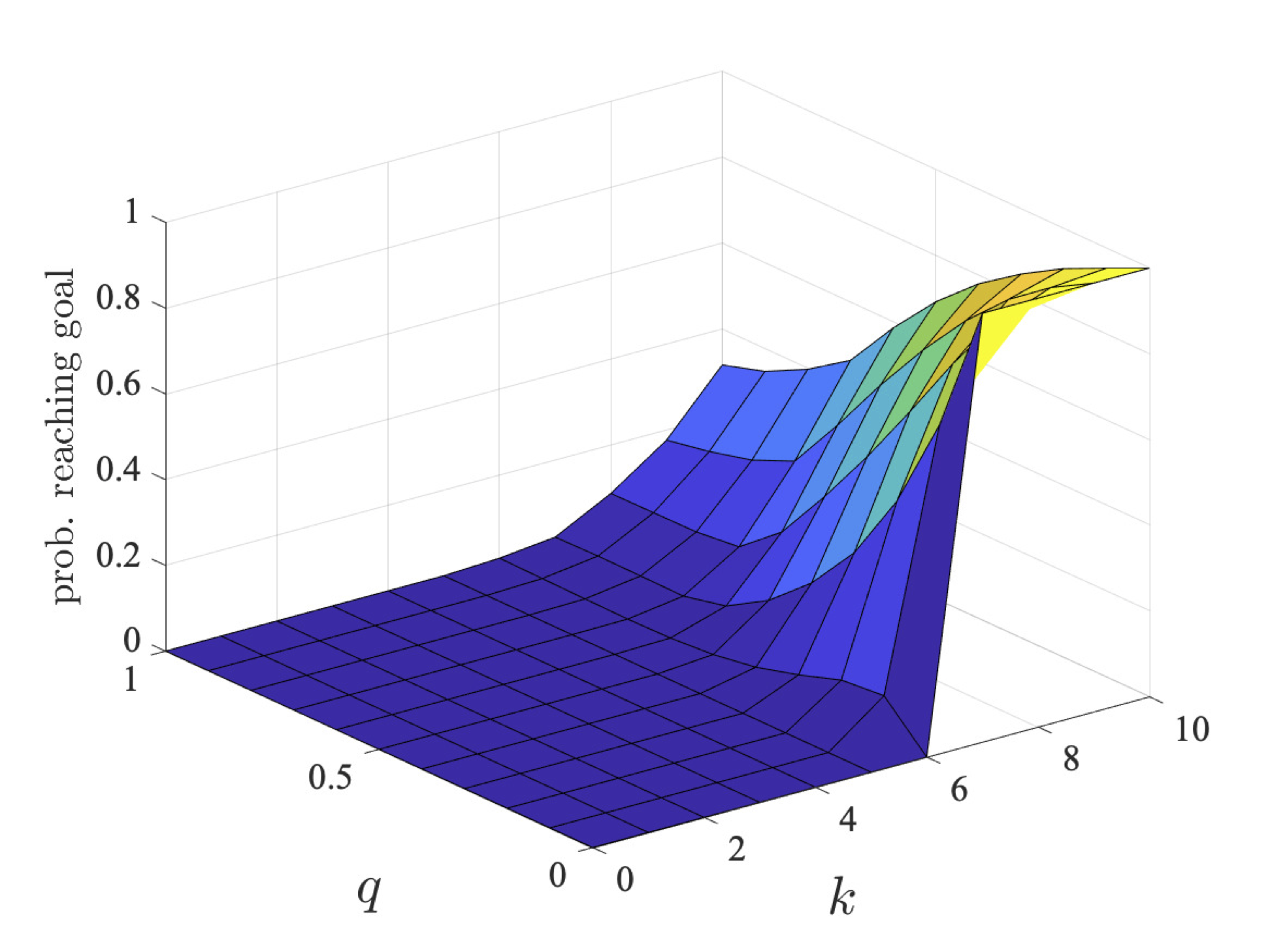
The graph below plots the results for the step-bounded variant of the same property as q and k vary for l=3, 5 and 7.
The graph below plots the results for expected reachability as l and q vary.
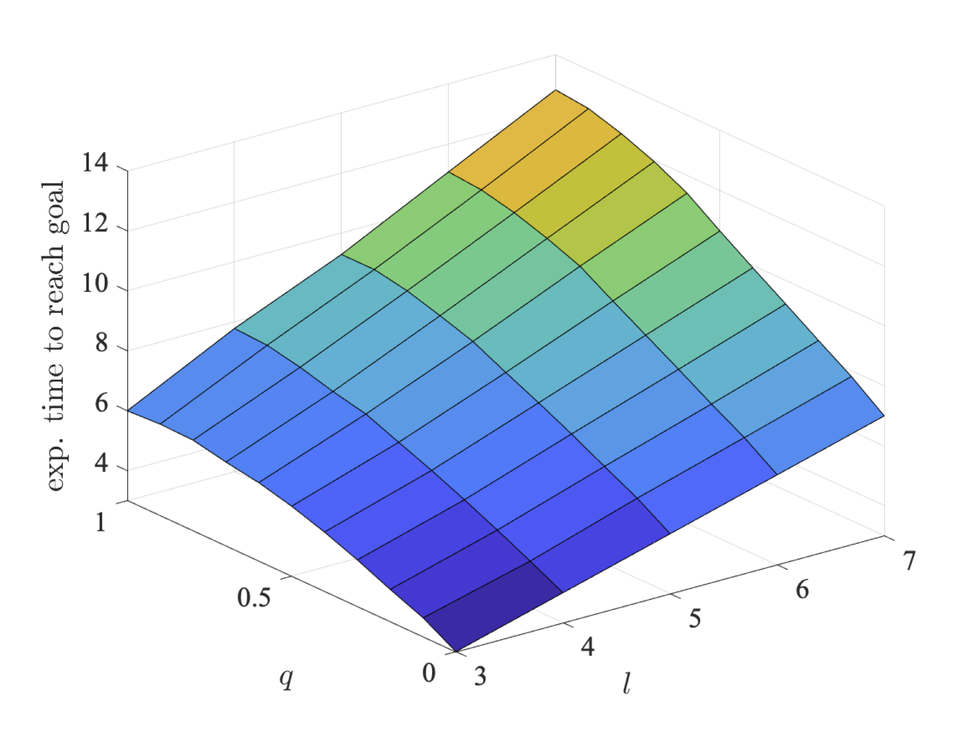
Again we see that increasing the size of the grid decreases the chance of crashing, and therefore increases the probability of reaching the goal within a deadline. The expected time increases as increasing the size of the grid means that more steps are required to reach the goal.
We next consider non-zero-sum properties where both players (robots) try and reach their individual goals. For this, we synthesise strategies that are social-welfare Nash equilibria (SWNE) [KNPS19]. Again we consider three classes of properties:
const int k; // step bound

// robots try to maximise the probability of reaching their goals without crashing
<<robot1:robot2>>max=? (P[ !"crash" U "goal1" ] + P[ !"crash" U "goal2" ])

// robots try to maximise the probability of reaching their goals without crashing within a bounded number of steps
<<robot1:robot2>>max=? (P[ !"crash" U<=k "goal1"] + P[ !"crash" U<=k "goal2"])

// robots try to maximise the probability of reaching their goals without crashing
// where the first one only has a bounded number of steps to do so
<<robot1:robot2>>max=? (P[!"crash" U<=k "goal1"] + P[!"crash" U "goal2"])

// robots try to minimise the expected time to reach their goals
<<robot1:robot2>>min=? (R{"time1"}[F "goal1" ] + R{"time2"}[F "goal2" ])
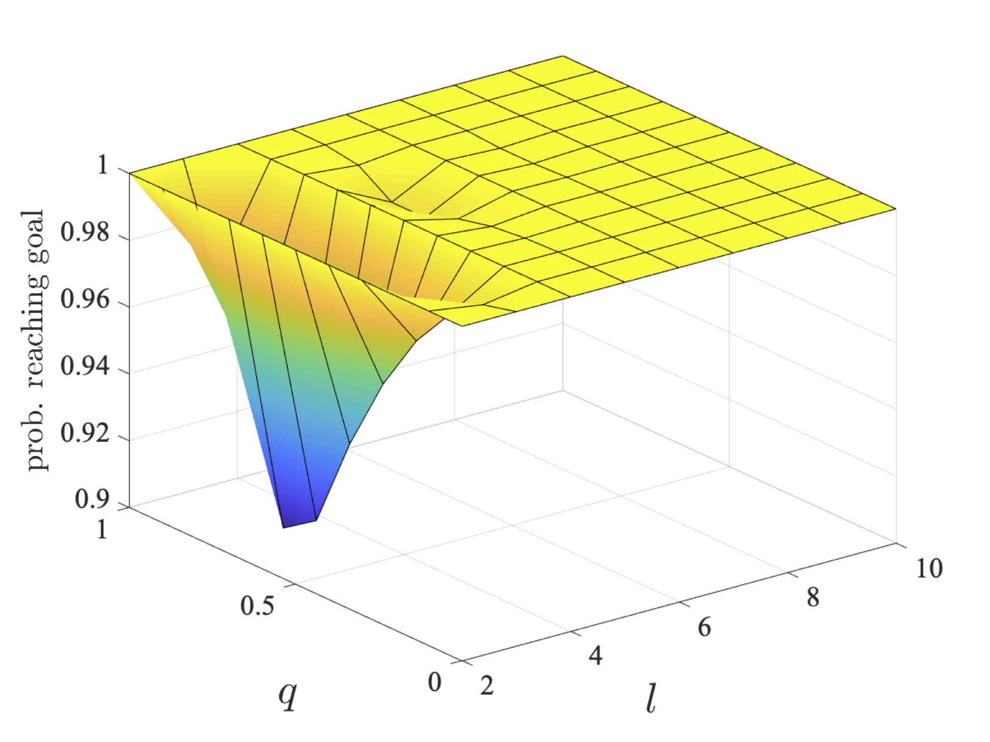
In the unbounded probabilistic reachability case, the optimal strategies allow each robot to reach its goal with a very high probability since, as time is not an issue, they can collaborate to avoid crashing and this also increases as the grid size increases as there is more room to avoid each other even with movement errors. The probability for odd sized grids is lower than for even sized grids, as for even sized grids the robots are more likely to jump over each other rather than landing in the same grid square. The graphs below plot the values of player 1 (left) and player 2 (right) as l and q vary.

For the step-bounded property, the graphs below show the probabilities for the individual players (player 1 left and player 2 right) as k and q vary, for l=3, 5 and 7.
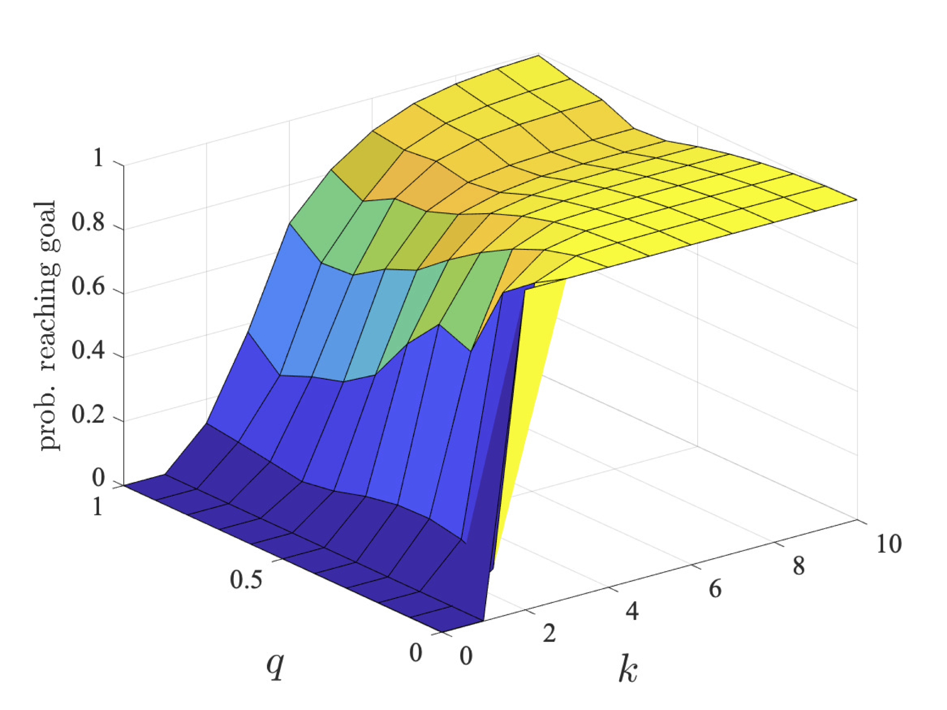
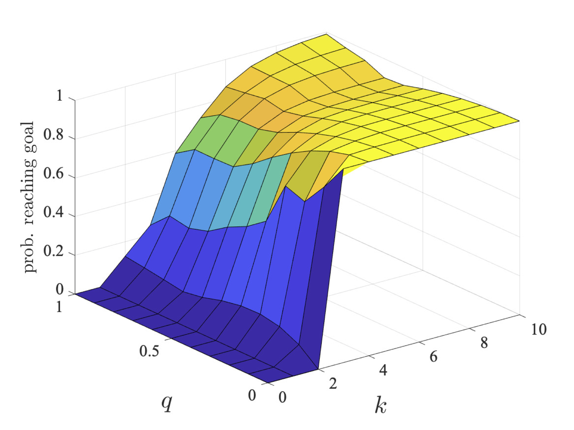
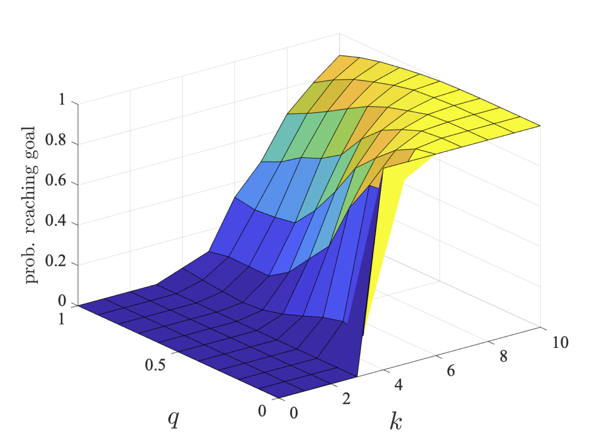
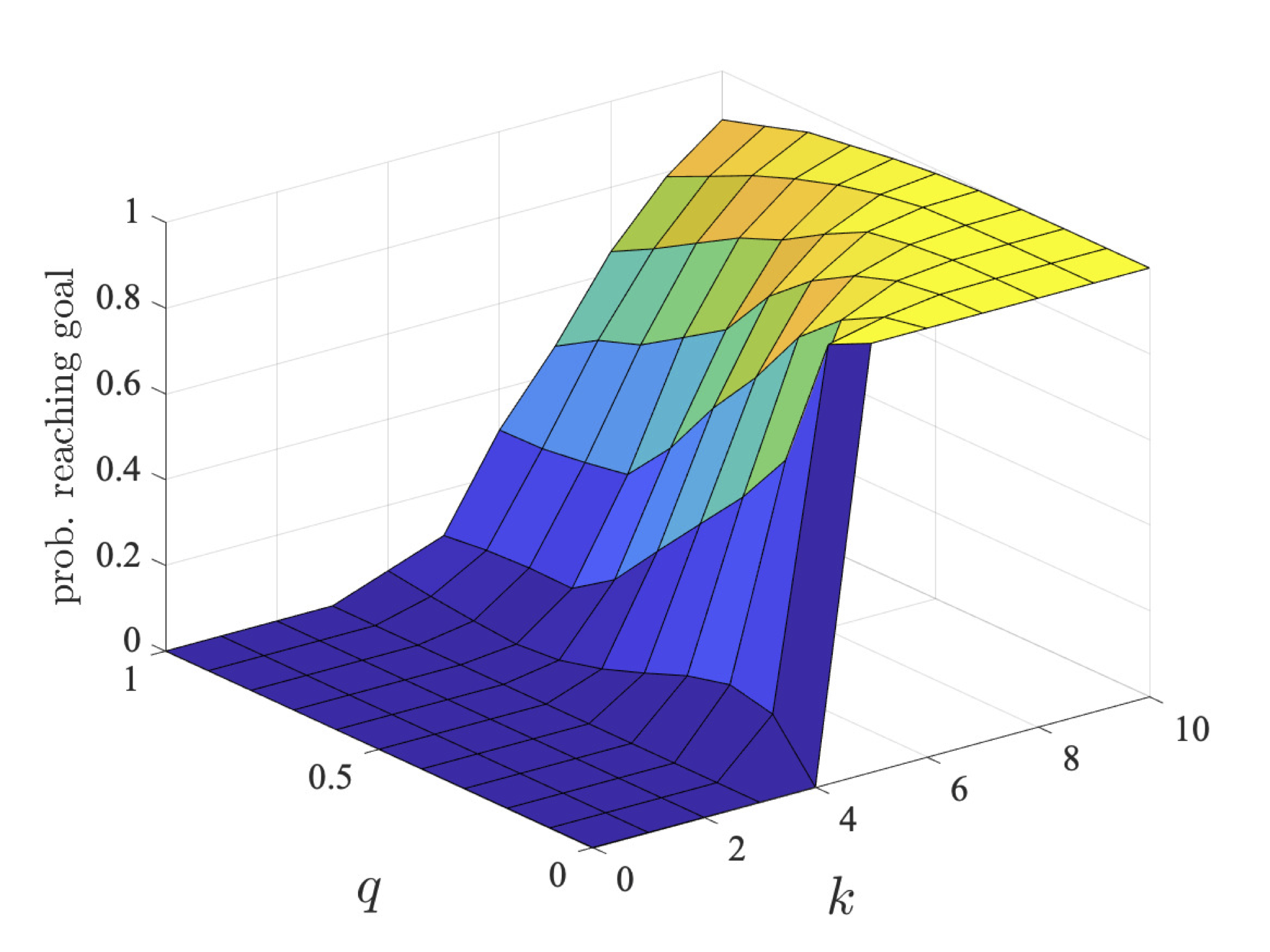
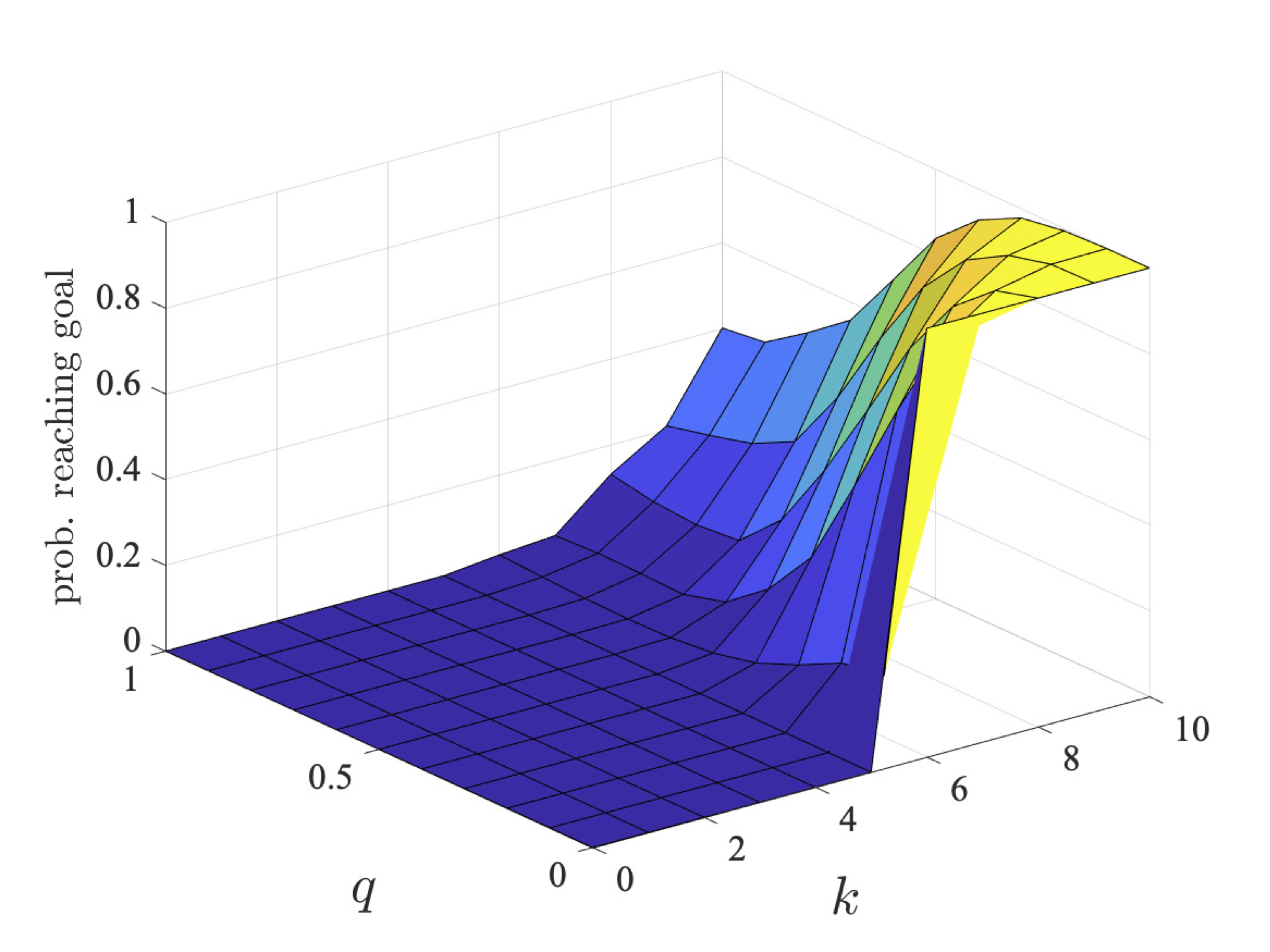
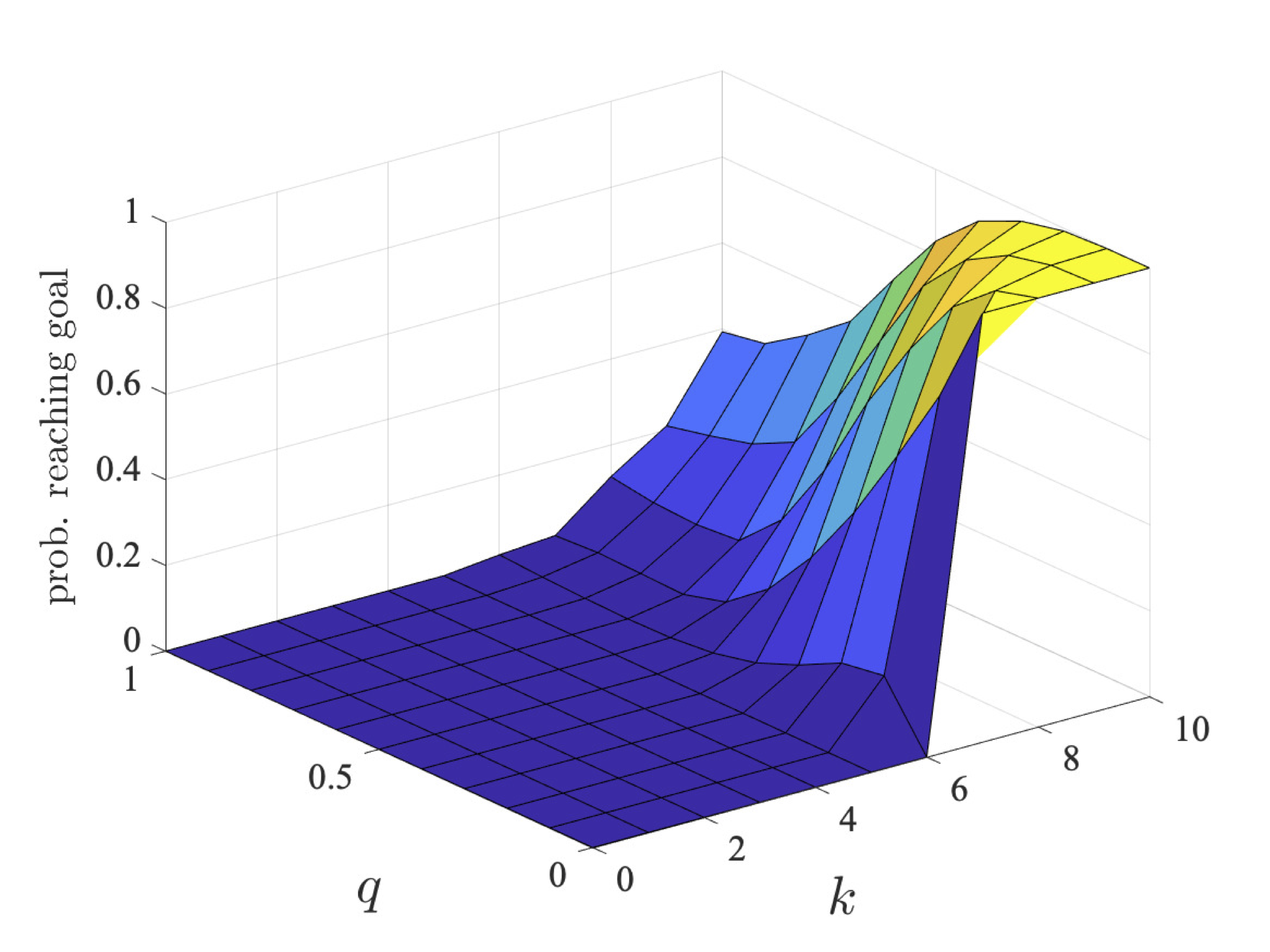
When there is only one route to each goal within the bound (along the diagonal), i.e. when k = l−1, the optimal strategies of both robots take this route as this is the only way of reaching the target within the deadline. In even grids, both players follow the diagonal route since, as discussed for the unbounded case, they will not crash but instead jump over each other. On the other hand, for odd grids, there is a high chance of crashing when they both follow the diagonal route, but there is also a chance one will deviate and the other reaches their goal. Initially, as the bound k increases, for odd grids the optimal values for the players are not equal. Here, it is better overall for one to follow the diagonal and the other to take a longer route, as if both took the diagonal route, the chance of crashing increases, decreasing the chance of reaching their goals.
The graph below plots the values of the individual players (player 1 left and player 2 right) for expected reachability as l and q vary.
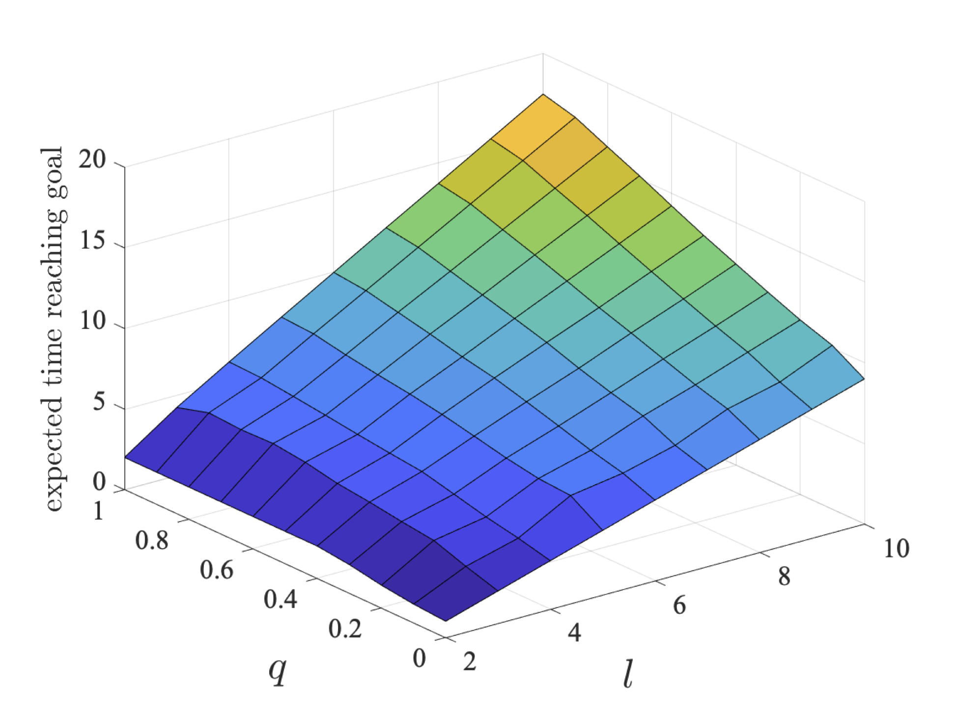
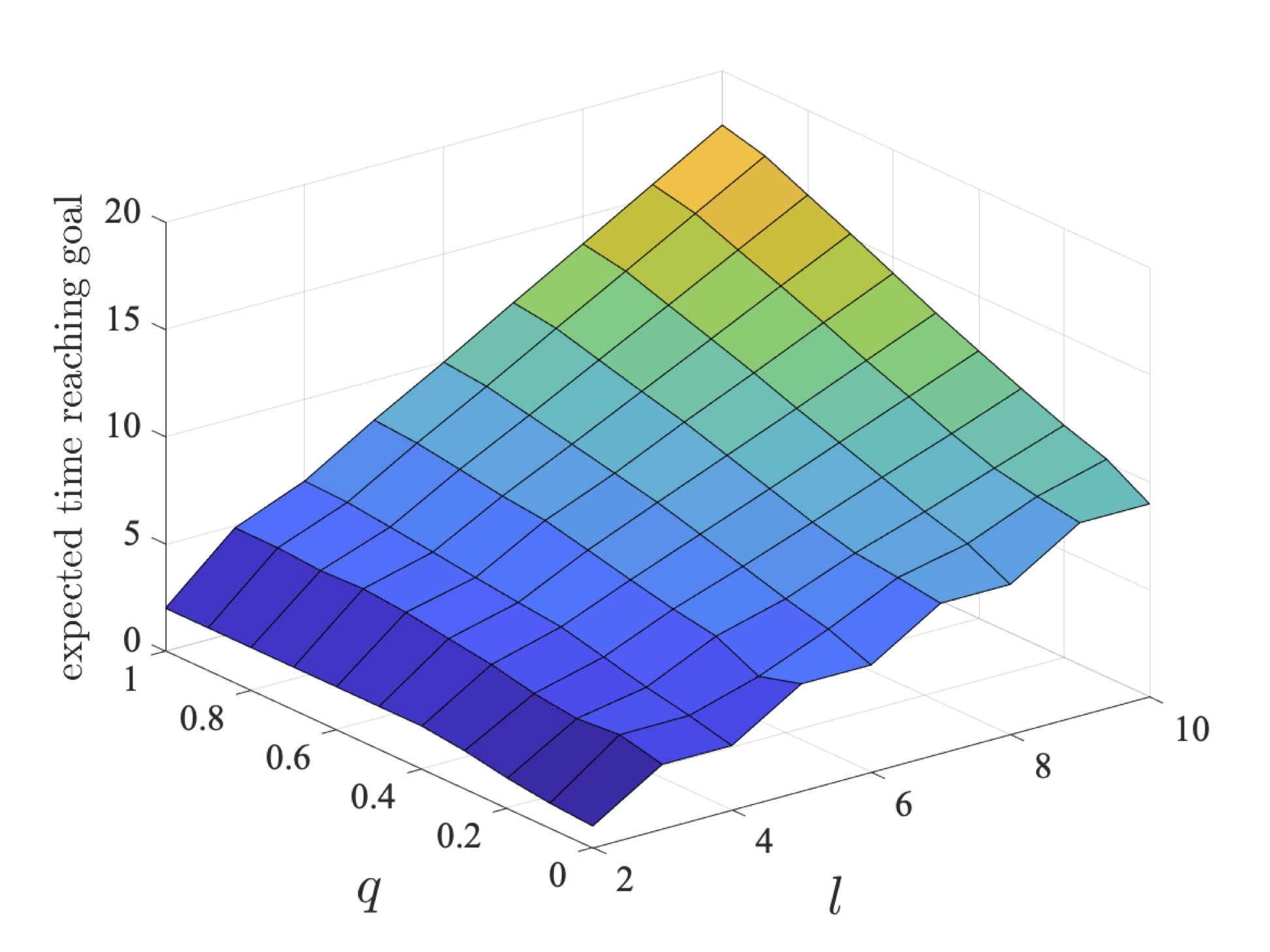
As for the deadline properties, we see that for odd grid sizes the values of the players are different for odd size grids. This is again due to the fact that if both players follow the (direct) diagonal route they will only crash for odd sized grids. The results again demonstrate that the players can gain by collaborating.