(Benini, Bogliolo, Paleologo and De Micheli)
This case study is based on a DTMC model of a IBM disk drive taken from [BBPM99]. As in [BBPM99] we suppose that the maximum size of the service request queue (SRQ) is 2.
The service provider (SP) has five different states which are shown below.
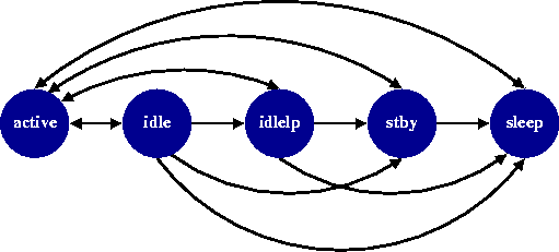
It is only in state active that the SP can perform data reads and writes. In state idle the disk is spinning while some of the electronic components of the disk drive have been switched off. The state idlelp (idle low power) is similar except that it has a lower power dissipation. The states stby and sleep correspond to the disk being spun down. The specification of the SP is given in the following tables.
Power Dissipation for states of the SP (W)
| active | 2.5 |
| idle | 1.5 |
| idlelp | 0.8 |
| stby | 0.3 |
| sleep | 0.1 |
Expected transition times for state transitions of the SP
| active | idle | idlelp | stby | sleep | |
| active | - | 1ms | 5ms | 2.2sec | 6sec |
| idle | 1ms | - | 5ms | 2.2sec | 6sec |
| idlelp | 5ms | - | - | 2.2sec | 6sec |
| stby | 2.2sec | - | - | - | 6sec |
| sleep | 6sec | - | - | - | - |
To model the system, we have chosen a time resolution of 1ms based on the fastest possible transition performed by the SP.
To model the PM issuing instructions to the SP, we split each time step of the system into two parts: in the first, the PM (instantaneously) decides what the SP should do next (based on the current state); and in the second, the system makes a transition (with the SP's move based on the choice made by the PM). To achieve this we include the following module:
module CLOCK

	c : [0..1];

	[tick1] c=0 -> (c'=1);
	[tick2] c=1 -> (c'=0);

endmodule
and construct the PM to synchronise with the CLOCK on tick1 and the remaining components of the system to synchronise with the clock on tick2.
Modelling the PM: As mentioned above the PM synchronises with the clock on tick1 and bases its choices on the current state of the system. Therefore the PM has the following form:
// POWER MANAGER

module PM

	pm  :  [0..4];
	// 0 - go to active
	// 1 - go to idle
	// 2 - go to idlelp
	// 3 - go to stby
	// 4 - go to sleep

	[tick1] cond1 -> p01 : (pm'=0) + p11 : (pm'=1) + p21 : (pm'=2) + p31 : (pm'=3) + p41 : (pm'=4);
	[tick1] cond2 -> p02 : (pm'=0) + p12 : (pm'=1) + p22 : (pm'=2) + p32 : (pm'=3) + p42 : (pm'=4);
	[tick1] cond3 -> p02 : (pm'=0) + p13 : (pm'=1) + p23 : (pm'=2) + p33 : (pm'=3) + p43 : (pm'=4);

endmodule
For example, if a state of the system satisfies cond1, then the PM decides that with probability p01 the SP moves to active, with probability p11 the SP moves to idle, with p21 to idlelp, p31 to stby, and p41 to sleep.
Modelling the SP: Recall that the SP synchronises with the clock on tick2 and the behaviour of the SP depends on the PM. Furthermore, since a time resolution of 1ms has been chosen, to correctly model transitions with delays longer than this time resolution, transient states are introduced. For example, the transient state active_idlelp is used to model the non-unitary time transition from active to idlelp. Note that, we suppose that the power dissipation in these transient states is high (2.5W). The module representing the SP has the following form:
// SERVICE PROVIDER

module SP

	sp : [0..10] init 9;
	// 0 active
	// 1 idle
	// 2 active_idlelp
	// 3 idlelp
	// 4 idlelp_active
	// 5 active_stby
	// 6 stby
	// 7 stby_active
	// 8 active_sleep
	// 9 sleep
	// 10 sleep_active

	// states where PM has no control (transient states)
	[tick2] sp=2  -> 0.75   : (sp'=2) + 0.25   : (sp'=3);  // active_idlelp
	[tick2] sp=4  -> 0.25   : (sp'=0) + 0.75   : (sp'=4);  // idlelp_active
	[tick2] sp=5  -> 0.995  : (sp'=5) + 0.005  : (sp'=6);  // active_stby
	[tick2] sp=7  -> 0.005  : (sp'=0) + 0.995  : (sp'=7);  // stby_active
	[tick2] sp=8  -> 0.9983 : (sp'=8) + 0.0017 : (sp'=9);  // active_sleep
	[tick2] sp=10 -> 0.0017 : (sp'=0) + 0.9983 : (sp'=10); // sleep_active

	// states where PM has control
	// goto_active
	[tick2] sp=0 & pm=0 -> (sp'=0); // active
	[tick2] sp=1 & pm=0 -> (sp'=0); // idle
	[tick2] sp=3 & pm=0 -> (sp'=4); // idlelp
	[tick2] sp=6 & pm=0 -> (sp'=7); // stby
	[tick2] sp=9 & pm=0 -> (sp'=10); // sleep
	// goto_idle
	[tick2] sp=0 & pm=1 -> (sp'=1); // active
	[tick2] sp=1 & pm=1 -> (sp'=1); // idle
	[tick2] sp=3 & pm=1 -> (sp'=3); // idlelp
	[tick2] sp=6 & pm=1 -> (sp'=6); // stby
	[tick2] sp=9 & pm=1 -> (sp'=9); // sleep
	// goto_idlelp
	[tick2] sp=0 & pm=2 -> (sp'=2); // active
	[tick2] sp=1 & pm=2 -> (sp'=2); // idle
	[tick2] sp=3 & pm=2 -> (sp'=3); // idlelp
	[tick2] sp=6 & pm=2 -> (sp'=6); // stby
	[tick2] sp=9 & pm=2 -> (sp'=9); // sleep
	// goto_stby
	[tick2] sp=0 & pm=3 -> (sp'=5); // active
	[tick2] sp=1 & pm=3 -> (sp'=5); // idle
	[tick2] sp=3 & pm=3 -> (sp'=5); // idlelp
	[tick2] sp=6 & pm=3 -> (sp'=6); // stby
	[tick2] sp=9 & pm=3 -> (sp'=9); // sleep
	// goto_sleep
	[tick2] sp=0 & pm=4 -> (sp'=8); // active
	[tick2] sp=1 & pm=4 -> (sp'=8); // idle
	[tick2] sp=3 & pm=4 -> (sp'=8); // idlelp
	[tick2] sp=6 & pm=4 -> (sp'=8); // stby
	[tick2] sp=9 & pm=4 -> (sp'=9); // sleep

endmodule
Modelling the SR and SRQ: As mentioned above, both the SRQ and the SR will synchronise with the clock on tick2. The SR has two states: idle, where no requests are generated; and 1req, where one request is generated per time step (1ms). The transitions between these states are based on time-stamped traces of disk access measured on real machines. The module of the SR is given by:
// SERVICE REQUESTER
module SR

	sr : [0..1] init 0; // 0 - idle and 1 - 1req

	[tick2] sr=0 -> 0.898: (sr'=0) + 0.102: (sr'=1);
	[tick2] sr=1 -> 0.454: (sr'=0) + 0.546: (sr'=1);

endmodule
In the case of the SRQ, to model the arrival and service of requests the transitions of the SRQ are dependent on the state of both the SR and the SP. Since, either the SR is in state idle and no requests arrive or in state 1req and one request arrives, and the SP can only serve requests when it is in state active, the module of the SRQ is as given below:
// SERVICE REQUEST QUEUE
module SRQ

	q : [0..2] init 0;

	[tick2] sr=0 & sp>0 -> true; // do not serve and nothing arrives
	[tick2] sr=1 & sp>0 -> (q'=min(q+1,2)); // do not serve and a request arrives
	[tick2] sr=0 & sp=0 -> (q'=max(q-1,0)); // serve and nothing arrives
	[tick2] sr=1 & sp=0 -> true; // serve and a request arrives arrives

endmodule
Reward Structures: We include the following reward structures for the power consumption, queue size and number of lost requests.
// power consumption
rewards "power"

	sp=0 & c=1 : 2.5;
	sp=1 & c=1 : 1.5;
	sp=2 & c=1 : 2.5;
	sp=3 & c=1 : 0.8;
	sp=4 & c=1 : 2.5;
	sp=5 & c=1 : 2.5;
	sp=6 & c=1 : 0.3;
	sp=7 & c=1 : 2.5;
	sp=8 & c=1 : 2.5;
	sp=9 & c=1 : 0.1;
	sp=10 & c=1 : 2.5;

endrewards

// queue size
rewards "queue"

	c=1 : q;

endrewards

// customers lost
rewards "lost"

	[tick2] q=2 & sr=1 & sp>0 : 1;

endrewards

// time
rewards "time"

    [tick2] true : 1;

endrewards
The policies we have calculated are the optimum policies for minimizing power consumption under different performance constraints, where these constraints concern the average number of requests awaiting service. In addition, we suppose that there is a time horizon of one million time steps. To model this horizon we include an additional module representing a battery which has an expected life span of 1 million time steps.
// BATTERY
module BAT

	bat : [0..1] init 1; // 0 empty, 1 - operational

	[] bat=0 -> (bat'=0); // loop when battery empty
	[tick2] bat=1 -> 0.000001 : (bat'=0) + 0.999999 : (bat'=1);

endmodule
Note that, once the battery reaches state 0 it cannot perform the action tick2 which prevents the rest of the system performing the action tick2, and hence prevents the rest of the system from moving (i.e. the states where bat=0 act as sink states).
We obtained these policies by constructing the generator matrix of the system in PRISM and then, from this, constructing a linear optimization problem which we solve with Maple using its Simplex package.
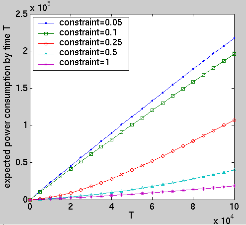
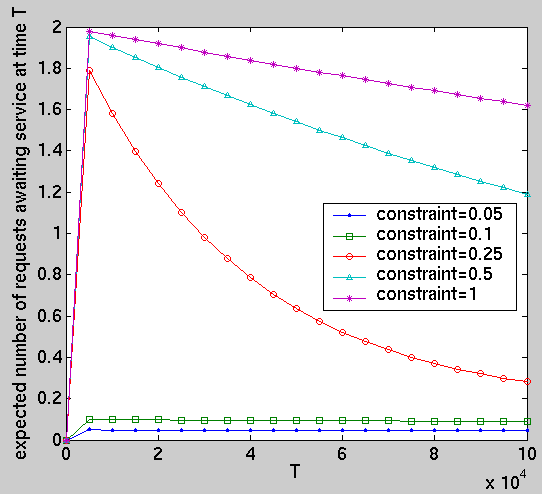
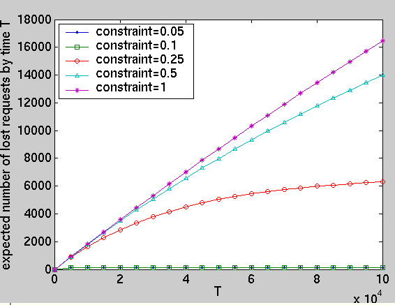
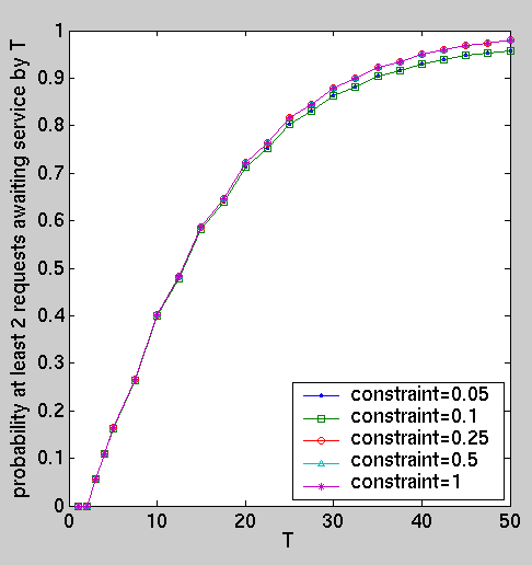
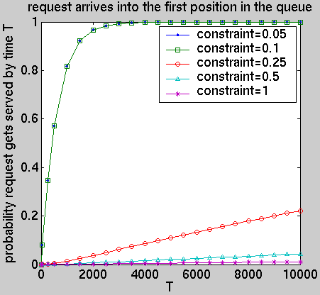
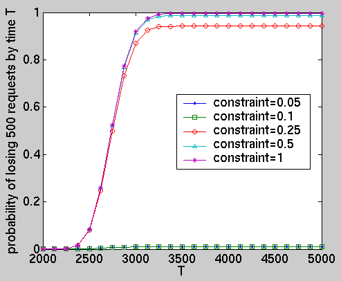
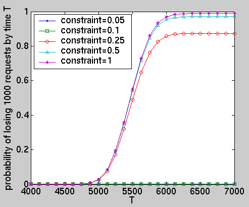
We have computed the following performance measures for the optimal policies under different constraints:
The above properties can be represented in the PRISM specification language as follows.
const int T; // time
const int K; // queue size

// average power consumption
R{"power"}=?[ F (bat=0) ]/R{"time"}=?[ F (bat=0) ]

// average queue size
R{"queue"}=?[ F (bat=0) ]/R{"time"}=?[ F (bat=0) ]

// average number of lost requests
R{"lost"}=?[ F (bat=0) ]/R{"time"}=?[ F (bat=0) ]

// the expected power consumption by time T
R{"power"}=?[ C<=2*T ]

// the expected number of requests awaiting service at time T .
R{"queue"}=?[ I=2*T ]

// the expected number of lost requests by time T .
R{"lost"}=?[ C<=2*T ]

// probability queue of size k before time T
P=?[ F q=K ]
The remaining properties below, reduce to calculating reachability probabilities after augmenting the model with a variable to record the property of interest.


