(Q. Zhu and T. Başar)
Related publications: [KNPS18]
In [ZB09], CSGs are used to model the interaction between an intrusion detection policy and attacker. The policy has a number of libraries that it can use to detect attacks and the attacker has several different attacks which can incur different levels of damage if not detected. Furthermore, each library can only detect certain attacks. In the model, in each round, the policy chooses a library to deploy and the attacker chooses an attack. A reward structure is specified representing the level of damage when an attack is not detected. The goal is to find optimal intrusion detection policies which correspond to finding a strategy for the policy that minimises damage.
For such systems, concurrency is required for the model to be meaningful, otherwise it is easy for the player whose turn follows the other player’s to 'win'. For example, if the attacker knows what library is being deployed, then it can simply choose an attack the library cannot detect.
We first present a simple model and then extend this model to the two scenarios presented in [ZB09] which we then analyse.
We first consider a simple CSG where the attacker can choose two different attacks and the defender can choose between defences for the two different attacks. The system can be in one of two states: healthy or compromised. The system starts in the healthy state and, if the correct defence for an attack is chosen, then the system remains or returns to this state; if the wrong defence is chosen for am attack, the system remains or moves to the compromised state.
Each time the wrong defence is chosen, a cost is incurred for the system. This cost is larger if the system was already in the compromised state when the wrong defence was chosen.
The CSG model is given below. There are two players: the attacker and the intrusion detection policy, and each has a single module which allows the player to choose the attack or defence for the current round. There are two additional modules not under the control of any player. The first counts the number of rounds. The round counter increases no matter what actions the players choose and therefore the commands of this model are unlabelled. The second module is used to keep track of the state of the system. Since the state of the system depends on whether the correct defence was chosen, in this module the commands are labelled by the choices of the two players.
The CSG also includes two reward structures. The first gives the cost incurred by the system in each round, while the second gives the cost in a specific round. If the correct defence is chosen, then there is no cost to the system. On the other hand, if the defence does not match the cost there is a cost. We assume that the second defence has limited success defending the first attack, while the first has no influence on the second, and therefore the cost is larger when choosing the first defence against the second attack.
// Intrusion detection system taken from
// Dynamic Policy-Based IDS Configuration
// Quanyan Zhu and Tamer Basar
// gxn 20/03/18

// simple example from the paper with 2 libraries and attacks
// and system can only be healthy or compromised

csg

player policy policy endplayer
player attacker attacker endplayer

const int rounds;

module rounds

	r : [0..rounds]; // current time-step

	[] r<rounds -> (r'=r+1);
	[] r=rounds -> true;

endmodule

module csystem

	s : [1..2]; // system state
	// 1 - healthy
	// 2 - compromised

	[defend1,attack1] true -> (s'=1);
	[defend1,attack2] true -> (s'=2);
	[defend2,attack1] true -> (s'=2);
	[defend2,attack2] true -> (s'=1);

endmodule

module policy

	[defend1] r<rounds -> true;
	[defend2] r<rounds -> true;

endmodule

module attacker

	[attack1] r<rounds -> true;
	[attack2] r<rounds -> true;

endmodule

rewards "damage"
	[defend1,attack1] s=1 : 0;
	[defend1,attack2] s=1 : 1;
	[defend2,attack1] s=1 : 0.5;
	[defend2,attack2] s=1 : 0;
	[defend1,attack1] s=2 : 1;
	[defend1,attack2] s=2 : 2;
	[defend2,attack1] s=2 : 1.5;
	[defend2,attack2] s=2 : 1;
endrewards

const K;

rewards "i_damage"
	[defend1,attack1] r=K-1 & s=1 : 0;
	[defend1,attack2] r=K-1 & s=1 : 1;
	[defend2,attack1] r=K-1 & s=1 : 0.5;
	[defend2,attack2] r=K-1 & s=1 : 0;
	[defend1,attack1] r=K-1 & s=2 : 1;
	[defend1,attack2] r=K-1 & s=2 : 2;
	[defend2,attack1] r=K-1 & s=2 : 1.5;
	[defend2,attack2] r=K-1 & s=2 : 1;
endrewards
We now extend the above model to the two scenarios given in [ZB09]. The system now has 3 possible states: healthy, compromised and failure. The system starts in the healthy state and transitions between states depending on whether the correct or wrong defence is chosen. In addition, the reward structures are extended so that the cost of a successful attack is greater when in the failure state than in the compromised state.
In the healthy state:
In the compromised state:
In the failure state:
The PRISM code for this CSG is below.
// intrusion detection CSG model taken from
// Dynamic Policy-Based IDS Configuration
// Quanyan Zhu and Tamer Basar
// gxn 20/03/18

const int scenario; // 1 or 2

// scenario 1:
// - small chance an attack is successful
// - high chance of recovering to healthy if attack is prevented
// - small chance of failure from compromised state (if attack continues)
// - high change that we repair from failure to compromised when attack stops

// scenario 2:
// - high chance an attack is successful
// - small chance of recovering to healthy if attack is prevented
// - high chance of failure from compromised state (if attack continues)
// - small change that we repair from failure to compromised when attack stops

const double attack = scenario=1 ? 0.2 : 0.8;
const double recover = scenario=1 ? 0.8 : 0.2;
const double fail = scenario=1 ? 0.2 : 0.8;
const double repair = scenario=1 ? 0.8 : 0.2;

csg

player policy policy endplayer
player attacker attacker endplayer

const int rounds; // number of rounds

module rounds

	r : [0..rounds]; // current time-step

	[] r<rounds -> (r'=r+1);
	[] r=rounds -> true;

endmodule

module csystem

	s : [1..3]; // system state
	// 1 - healthy
	// 2 - compromised
	// 3 - failure

	[defend1,attack1] s=1 -> (s'=1);
	[defend1,attack2] s=1 -> 1-attack : (s'=1) + attack : (s'=2);
	[defend2,attack1] s=1 -> 1-attack : (s'=1) + attack : (s'=2);
	[defend2,attack2] s=1 -> (s'=1);

	[defend1,attack1] s=2 -> recover : (s'=1) + 1-recover : (s'=2);
	[defend1,attack2] s=2 -> 1-fail : (s'=2) + fail : (s'=3);
	[defend2,attack1] s=2 -> 1-fail : (s'=2) + fail : (s'=3);
	[defend2,attack2] s=2 -> recover : (s'=1) + 1-recover : (s'=2);

	[defend1,attack1] s=3 -> repair : (s'=2) + 1-repair : (s'=3);
	[defend1,attack2] s=3 -> (s'=3);
	[defend2,attack1] s=3 -> (s'=3);
	[defend2,attack2] s=3 -> repair : (s'=2) + 1-repair : (s'=3);

endmodule

module policy

	[defend1] r<rounds -> true;
	[defend2] r<rounds -> true;

endmodule

module attacker

	[attack1] r<rounds -> true;
	[attack2] r<rounds -> true;

endmodule

rewards "damage"
	[defend1,attack1] s=1 : 0;
	[defend1,attack2] s=1 : 1;
	[defend2,attack1] s=1 : 0.5;
	[defend2,attack2] s=1 : 0;
	[defend1,attack1] s=2 : 1;
	[defend1,attack2] s=2 : 2;
	[defend2,attack1] s=2 : 1.5;
	[defend2,attack2] s=2 : 1;
	[defend1,attack1] s=3 : 1;
	[defend1,attack2] s=3 : 3;
	[defend2,attack1] s=3 : 2.5;
	[defend2,attack2] s=3 : 1;
endrewards

const K;

rewards "i_damage"
	[defend1,attack1] r=K-1 & s=1 : 0;
	[defend1,attack2] r=K-1 & s=1 : 1;
	[defend2,attack1] r=K-1 & s=1 : 0.5;
	[defend2,attack2] r=K-1 & s=1 : 0;
	[defend1,attack1] r=K-1 & s=2 : 1;
	[defend1,attack2] r=K-1 & s=2 : 2;
	[defend2,attack1] r=K-1 & s=2 : 1.5;
	[defend2,attack2] r=K-1 & s=2 : 1;
	[defend1,attack1] r=K-1 & s=3 : 1;
	[defend1,attack2] r=K-1 & s=3 : 3;
	[defend2,attack1] r=K-1 & s=3 : 2.5;
	[defend2,attack2] r=K-1 & s=3 : 1;
endrewards
We consider two scenarios, where in scenario 1:
and in scenario 2:
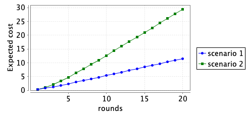
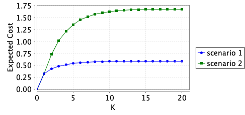
For the two scenarios given above we consider both the cumulated cost over a number of rounds and the cost of a specific round.
// minimum cumulative expected damage the IDS policy can enforce
<<policy>> R{"damage"}min=? [F r=rounds ]

// minimum expected damage the IDS policy can enforce in round K
<<policy>> R{"i_damage"}min=? [ F r=K ]
The two graphs below plot the minimum expected cumulative cost over a number of rounds and the minimum expected cost in a specific round that the policy player can ensure.


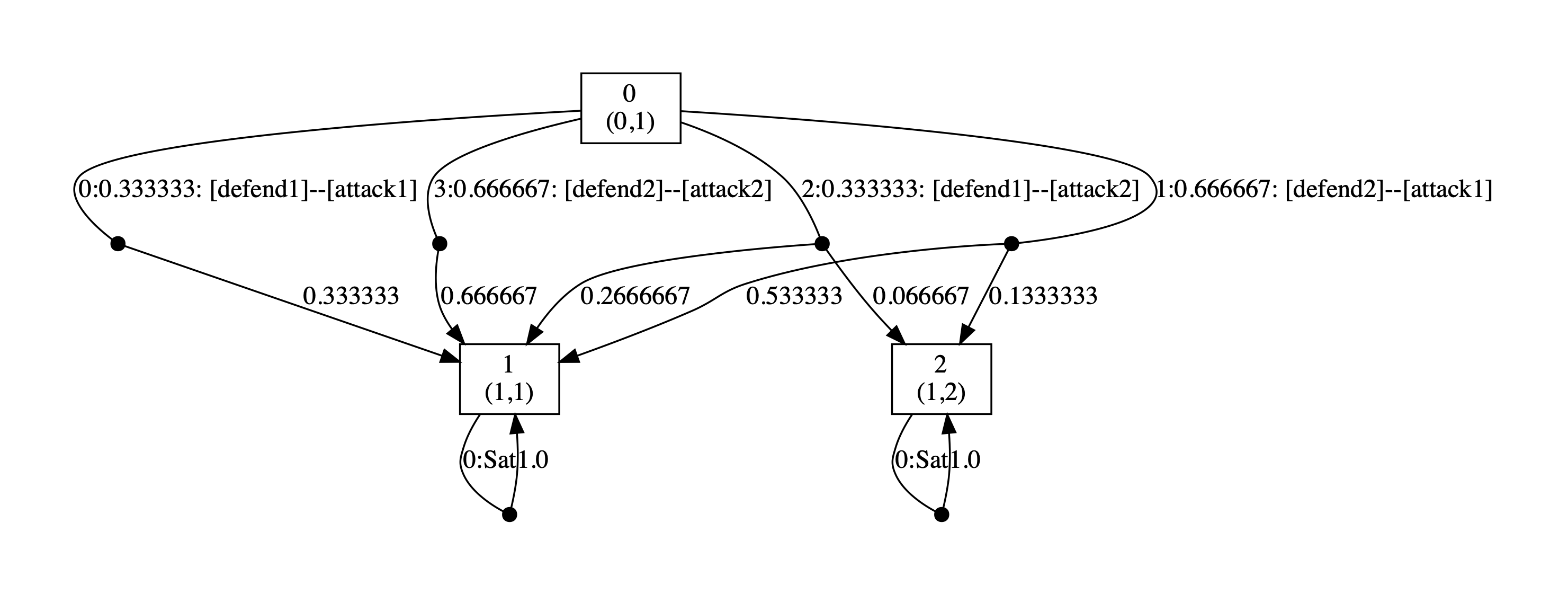
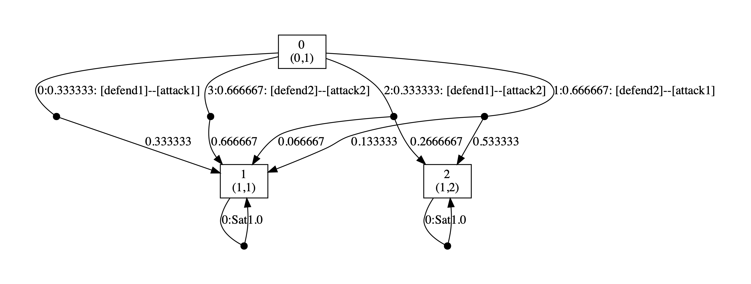
We also synthesise the optimal strategy for the defender over 1, 2 and 4 rounds. For example, for the first scenario and when the number of rounds is 2, this is achieved through the following command:
Below we have included the generated optimal strategies for the defender. In the graph, the vertices correspond to the states of the game, i.e. the values of the variables rounds and s, and edges from any state represent the optimal choices of player 1 and all available choices for player 2 from that state. The choices for the two players (probability of choosing available actions) are separated by --. By including all possible choices for player 2, the graph includes all states reachable when player 1 follows its optimal strategy, and therefore all choices for this strategy when it is followed.
As the graphs below demonstrate, the optimal strategy for the defender is in each case randomised. In addition, it favours the second defence which can be attributed to the fact that the second defence has at least partial success against both attacks while this is not true of the first.


